K nearest Neighbor (kNN) exercise
- training 과정에서 classifier은 단순히 training data를 기억할 것이다.
- testing 과정에서 classifier은 각각의 test 이미지를 모든 training 이미지와 비교해서 그 중가장 가까운 k개의 training 이미지의 label로 결정할 것이다.
- k의 값은 cross-validation 과정을 통해 결정된다.
1. code setup, import data and packages
# Run some setup code for this notebook.

import random
import numpy as np
from cs231n.data_utils import load_CIFAR10
import matplotlib.pyplot as plt

# This is a bit of magic to make matplotlib figures appear inline in the notebook
# rather than in a new window.
%matplotlib inline
plt.rcParams['figure.figsize'] = (10.0, 8.0) # set default size of plots
plt.rcParams['image.interpolation'] = 'nearest'
plt.rcParams['image.cmap'] = 'gray'

# Some more magic so that the notebook will reload external python modules;
# see http://stackoverflow.com/questions/1907993/autoreload-of-modules-in-ipython
%load_ext autoreload
%autoreload 2

# Load the raw CIFAR-10 data.
cifar10_dir = 'cs231n/datasets/cifar-10-batches-py'

# Cleaning up variables to prevent loading data multiple times (which may cause memory issue)
try:
   del X_train, y_train
   del X_test, y_test
   print('Clear previously loaded data.')
except:
   pass

X_train, y_train, X_test, y_test = load_CIFAR10(cifar10_dir)
필요한 패키지들을 불러오고 plot을 그릴 때 기본 설정들을 해주었고 cifar-10 데이터셋에서 필요한 데이터들을 불러왔다.
Training data shape: (50000, 32, 32, 3)
Training labels shape: (50000,)
Test data shape: (10000, 32, 32, 3)
Test labels shape: (10000,)
2. class 별로 이미지 확인하기
# Visualize some examples from the dataset.
# We show a few examples of training images from each class.
classes = ['plane', 'car', 'bird', 'cat', 'deer', 'dog', 'frog', 'horse', 'ship', 'truck']
num_classes = len(classes)
samples_per_class = 7
for y, cls in enumerate(classes):
    idxs = np.flatnonzero(y_train == y)
    idxs = np.random.choice(idxs, samples_per_class, replace=False)
    for i, idx in enumerate(idxs):
        plt_idx = i * num_classes + y + 1
        plt.subplot(samples_per_class, num_classes, plt_idx)
        plt.imshow(X_train[idx].astype('uint8'))
        plt.axis('off')
        if i == 0:
            plt.title(cls)
plt.show()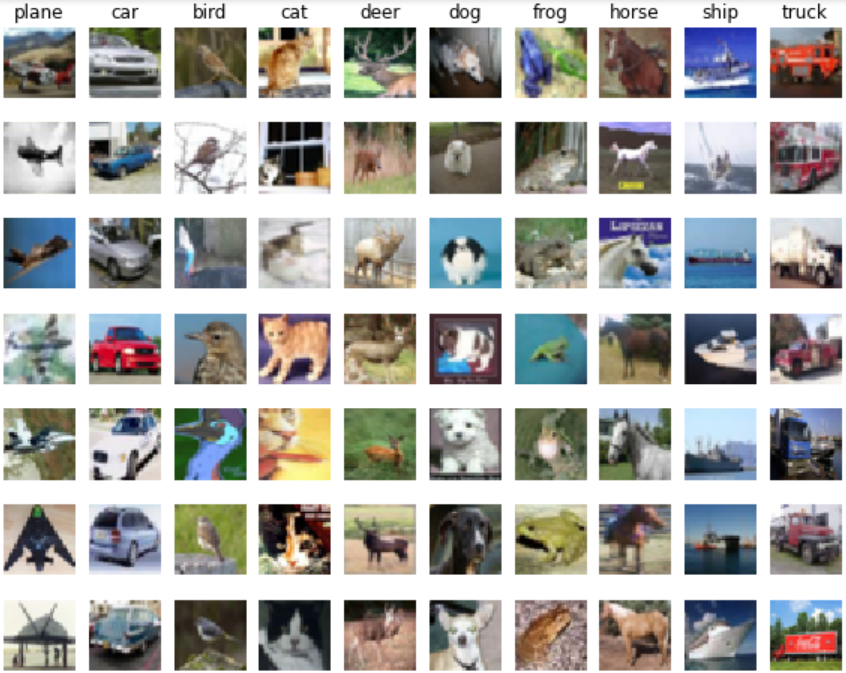
class는 plane부터 truck까지 10종류가 있고, 각 class당 7개의 example 사진들을 불러왔다.
3. 일부 데이터를 reshape
# Subsample the data for more efficient code execution in this exercise
num_training = 5000
mask = list(range(num_training))
X_train = X_train[mask]
y_train = y_train[mask]

num_test = 500
mask = list(range(num_test))
X_test = X_test[mask]
y_test = y_test[mask]

# Reshape the image data into rows
X_train = np.reshape(X_train, (X_train.shape[0], -1))
X_test = np.reshape(X_test, (X_test.shape[0], -1))
print(X_train.shape, X_test.shape)
(5000, 3072) (500, 3072)
모델 훈련의 편의성을 위해 train, test set에서 각각 5000개, 500개의 data만을 불러왔다.
(50000개 중 5000개의 데이터를 선택하는 과정은 random하게 하지 않고 앞쪽의 5000개를 mask로 불러온 것이다.)
왜 random으로 선택하지 않았을까? 애초에 training, test set 자체가 random하게 배열되어 있나?
또한, 하나의 이미지에 대한 pixel 값들을 하나의 벡터 형태로 길게 펴주었다.
4. kNN 모델 학습
from cs231n.classifiers import KNearestNeighbor

# Create a kNN classifier instance.
# Remember that training a kNN classifier is a noop:
# the Classifier simply remembers the data and does no further processing
classifier = KNearestNeighbor()
classifier.train(X_train, y_train)
cs231n에서 knn 모델을 불러와서 x train과 y train으로 모델을 학습했다.
5. distance 구하기: compute_distances_two_loops
k_nearest_neighbor.py에서 compute_distances_two_loops 함수로 두번의 루프를 돌아 test set과 train set 사이의 거리를 L2 distance로 계산하겠다.
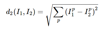
(test set 개수 * train set 개수)의 shape을 가진 dists라는 array 안에, (i,j) 요소는 i번째 test example이 j번째 train example과의 L2 distance가 계산될 것이다.
k_nearest_neighbor.py
from builtins import range
from builtins import object
import numpy as np
from past.builtins import xrange


class KNearestNeighbor(object):

    def __init__(self):
        pass

    def train(self, X, y):
        self.X_train = X
        self.y_train = y

    def predict(self, X, k=1, num_loops=0):
        if num_loops == 0:
            dists = self.compute_distances_no_loops(X)
        elif num_loops == 1:
            dists = self.compute_distances_one_loop(X)
        elif num_loops == 2:
            dists = self.compute_distances_two_loops(X)
        else:
            raise ValueError('Invalid value %d for num_loops' % num_loops)

        return self.predict_labels(dists, k=k)

    def compute_distances_two_loops(self, X):
        ...
        return dists

    def compute_distances_one_loops(self, X):
        ...
        return dists

    def compute_distances_no_loops(self, X):
        ...
        return dists

    def predict_labels(self, dists, k=1):
        ...
        return y_pred
k_nearest_neighbor.py에 담긴 KNearestNeighboor 클래스의 기본 골자는 다음과 같다. 4의 kNN 모델 학습에서 kNN 클래스의 train 함수가 사용되었고 2개 또는 1개 또는 0개의 loop로 dists를 계산하고 계산한 dists로 test set의 label을 predict 할 것이다.
compute_distances_two_loops
def compute_distances_two_loops(self, X):
    num_test = X.shape[0]
    num_train = self.X_train.shape[0]
    dists = np.zeros((num_test, num_train))
    for i in range(num_test):
        for j in range(num_train):
            dists[i,j]=np.sqrt(np.sum((X[i,:]-self.X_train[j,:])**2))
X(test)의 i번째 행에 i번째 example의 pixel이, X_train의 j번째 행에 j번째 example의 pixel이 담겨있다. 이를 빼주고, 제곱해주고, 합쳐주고, 제곱근을 계산하면 두 example의 distance가 된다.
dists = classifier.compute_distances_two_loops(X_test)
print(dists.shape)  #(500, 5000)

plt.imshow(dists, interpolation='none')
plt.show()
X_test에 대해 compute_distances_two_loops로 dists array를 만들어줬고, 행 수가 test 개수인 500, 열 수가 train 개수인 5000임을 확인했다.
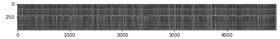
dists를 시각화한 것인데, 세로축은 test set, 가로축은 train set에 해당한다. 검정색일 수록 example 간 거리가 멀어서 dists의 값이 크고 하얀색일수록 거리가 짧아서 dists의 값이 작다.
6. predict labels
predict_labels
def predict_labels(self, dists, k=1):
    num_test = dists.shape[0]
    y_pred = np.zeros(num_test)
    for i in range(num_test):
        closest_y = []

        s=np.argsort(dists[i,:])
        idx=s[:k]
        closest_y=self.y_train[idx]

        y_pred[i]=np.bincount(closest_y).argmax()

        return y_pred
x_test의 각 example에 대한 prediction 함수이다. dists의 i번째 행, 즉 i번째 test example에 대해 모든 train example과 dist를 계산한 행인 dists[i,:]에 대해 np.argsort()로 값이 작은 것부터 label을 불러온다. 이 label을 s변수에 저장했다.
e.x.)numpy.argsort(200,100,0,3)
=> 2,3,1,0으로, 가장 작은 값을 가진 label부터 차례로 돌려주는 함수이다.
가장 가까운 distance를 가진 k개의 training set을 가져오고 싶기 때문에 s의 앞에서부터 k개의 원소를 뽑아서 idx 변수에 저장한다.
이 training set의 label을 가져와야 하므로 y_train[idx]로 k개의 가장 가까운 y label을 closest_y에 저장한다.
np.bincount()로 가장 많이 나온 label 값의 빈도를 찾고, argmax()로 그 빈도의 index를 가져와서 y_pred에 저장한다.
# Now implement the function predict_labels and run the code below:
# We use k = 1 (which is Nearest Neighbor).
y_test_pred = classifier.predict_labels(dists, k=1)

# Compute and print the fraction of correctly predicted examples
num_correct = np.sum(y_test_pred == y_test)
accuracy = float(num_correct) / num_test
print('Got %d / %d correct => accuracy: %f' % (num_correct, num_test, accuracy))
k=1로 두고 (1-NN) predict_labels로 test set에 대한 y의 prediction을 가져와서 정확도를 예측했다.
Got 137 / 500 correct => accuracy: 0.274000
accuracy는 27.4%로 낮은 값이 나왔다.
y_test_pred = classifier.predict_labels(dists, k=5)
num_correct = np.sum(y_test_pred == y_test)
accuracy = float(num_correct) / num_test
print('Got %d / %d correct => accuracy: %f' % (num_correct, num_test, accuracy))
Got 139 / 500 correct => accuracy: 0.278000
k=5로 두고 정확도를 예측했더니 accuracy는 27.8%로 근소하게 높아졌다. k가 높아지면 test set에 대한 정확도가 상승한다.
7. 다른 방법으로 distance 구하고 비교하기
compute_distances_one_loops
 def compute_distances_one_loop(self, X):
    num_test = X.shape[0]
    num_train = self.X_train.shape[0]
    dists = np.zeros((num_test, num_train))
    for i in range(num_test):
        dists[i,:]=np.sqrt(np.sum((self.X_train-X[i,:])**2,axis=1).T)
    return dists
X_train은 (5000*D), X(test)[i,:]는 (1*D)의 shape을 가져서 둘을 빼주면 X(test)[i,:]가 (5000,D)로 broadcasting 돼서 모든 training example에 대해 하나의 test example의 차이가 구해지게 된다. 이 과정을 for문으로 모든 test examples에 대해 반복해주면 dists array를 얻을 수 있다.
dists_one = classifier.compute_distances_one_loop(X_test)

difference = np.linalg.norm(dists - dists_one, ord='fro')
print('One loop difference was: %f' % (difference, ))
if difference < 0.001:
    print('Good! The distance matrices are the same')
else:
    print('Uh-oh! The distance matrices are different')
One loop difference was: 0.000000
Good! The distance matrices are the same
compute_distances_one_loop로 X_test에 대한 dists를 구했고, 위에서 two_loop 함수로 구한 dists와 비교했더니 동일한 dists가 나옴을 확인했다.
compute_distances_no_loops
def compute_distances_no_loops(self, X):

        num_test = X.shape[0]
        num_train = self.X_train.shape[0]
        dists = np.zeros((num_test, num_train))

        a=np.dot(X,self.X_train.T)
        b=np.sum(X**2,axis=1).reshape((-1,1))
        c=np.sum((self.X_train.T)**2,axis=0)
        a=-2*a+b
        a=a+c
        dists=np.sqrt(a)

        return dists
test set의 i번째 행의 원소들을 i1, i2, i3, ... 라고 하고 train set의 j번째 행의 원소들을 j1, j2, j3, ...이라고 하자.
L2 distance의 (i,j)의 원소는 √(i1-j1)^2+(i2-j2)^2+(i3-j3)^2 ... 이고,
√(i1)^2 + (j1)^2 - 2*(i1)(j1) + (i2)^2 + (j2)^2 - 2*(i2)*(j2) + ...와 같다.
즉, √[(i1)^2 + (i2)^2 + (i3)^2 + ...] →1 + [(j1)^2 + (j2)^2 + (j3)^2 + ...] →2 - 2*[(i1)*(j1) + (i2)*(j2) + (i3)*(j3) + ...]→3와같다.
3→ np.dot(X(test), X_train.T)를 하면, (500*D)*(D*5000)=(500*5000)으로 각 원소들끼리 곱해진 형태로 구현할 수 있다.
1→ X(test)**2를 하면 모든 i들이 제곱형태가 되고 이를 np.sum()을 해주고, .reshape((-1,1)로 (500,D) 형태를 만든다.
2→ X_train.T**2를 하면 모든 j들이 제곱형태가 되고 이를 np.sum()을 해주면 (1*5000) 형태가 된다.
이렇게 1+2-2*3을 해주고 np.sqrt()까지 해줘서 dists array를 만들 수 있다.
dists_two = classifier.compute_distances_no_loops(X_test)

difference = np.linalg.norm(dists - dists_two, ord='fro')
print('No loop difference was: %f' % (difference, ))
if difference < 0.001:
    print('Good! The distance matrices are the same')
else:
    print('Uh-oh! The distance matrices are different')
No loop difference was: 0.000000
Good! The distance matrices are the same
이 또한 two loop으로 만든 dists와 동일한 dists가 만들어졌다.
dists 구하는 방법에 따른 시간 비교
def time_function(f, *args):
    import time
    tic = time.time()
    f(*args)
    toc = time.time()
    return toc - tic

two_loop_time = time_function(classifier.compute_distances_two_loops, X_test)
print('Two loop version took %f seconds' % two_loop_time)

one_loop_time = time_function(classifier.compute_distances_one_loop, X_test)
print('One loop version took %f seconds' % one_loop_time)

no_loop_time = time_function(classifier.compute_distances_no_loops, X_test)
print('No loop version took %f seconds' % no_loop_time)
Two loop version took 36.343373 seconds
One loop version took 28.159360 seconds
No loop version took 0.579636 seconds
loop가 없이 vectorization 될수록 시간이 짧게 걸린다.
Cross Validation
cross validation을 통해 최적의 k값을 찾아줄 것이다.
num_folds = 5
k_choices = [1, 3, 5, 8, 10, 12, 15, 20, 50, 100]

X_train_folds = []
y_train_folds = []

X_train_folds=np.array_split(X_train,num_folds)
y_train_folds=np.array_split(y_train,num_folds)

k_to_accuracies = {}

for k in k_choices:
  k_to_accuracies[k]=[]

for k in k_choices:
  for i in range(num_folds):
    X_train_folds=np.array_split(X_train,num_folds)
    y_train_folds=np.array_split(y_train,num_folds)
    X_cv_set=X_train_folds[i]
    y_cv_set=y_train_folds[i]
    del X_train_folds[i]
    del y_train_folds[i]
    X_train_set=np.array(X_train_folds).flatten().reshape(-1,X_train_folds[1].shape[1])
    y_train_set=np.squeeze(np.array(y_train_folds).flatten().reshape(1,-1))

    classifier = KNearestNeighbor()
    classifier.train(X_train_set, y_train_set)
    dists = classifier.compute_distances_no_loops(X_cv_set)

    y_cv_pred = classifier.predict_labels(dists, k=k)
    num_correct = np.sum(y_cv_pred == y_cv_set)
    accuracy = float(num_correct) / X_cv_set.shape[0]

    k_to_accuracies[k].append(accuracy)

for k in sorted(k_to_accuracies):
    for accuracy in k_to_accuracies[k]:
        print('k = %d, accuracy = %f' % (k, accuracy))
train set을 5개의 fold로 나눈 후, 각 fold별로 k_choices 안의 k값에 따른 성능을 구하고 그 때 accuracy를 k_to_accuracies에 넣을 것이다. 즉, 하나의 k값에 대해 fold1=cv일 때, fold2=cv일 때, ..., fold5=cv일 때의 accuracy를 모두 계산할 것이다.
X_train_folds는 5개의 array를 가진 list이고 하나의 array에는 1000개의 example이 포함되어 있다. 하나의 array를 cv로, 나머지 4개의 array를 train set으로 사용할 것이다.
y_train_folds 또한 5개의 array를 가진 list이고 cv와 train으로 쪼개줄 것이다.
X_train_set, y_train_set, X_cv_set, y_cv_set을 만들었다.
X_train_set은 X_train_folds에서 4개의 array를 선택한 뒤 flatten()으로 하나의 array로 만들어 주고, (4000*D)의 shape을 갖도록 reshape 해줬다.
y_train_set도 4개의 array를 flatten() 해주고 (1*4000)의 shape을 갖도록 reshape 해줬다. y_train_set[0]에서 비로소 1*4000의 shape을 갖기에 np.squeeze도 해줬다.
knn으로 train 해주고 dists를 생성하고 prediction을 한 뒤 accuracy를 계산하고 그 값을 k_to_accuracies 딕셔너리에 추가하고 그 값들을 출력했다.
k = 1, accuracy = 0.263000
k = 1, accuracy = 0.257000
k = 1, accuracy = 0.264000
k = 1, accuracy = 0.278000
k = 1, accuracy = 0.266000
.....
k = 100, accuracy = 0.256000
k = 100, accuracy = 0.270000
k = 100, accuracy = 0.263000
k = 100, accuracy = 0.256000
k = 100, accuracy = 0.263000
한눈에 보기 위해 plot으로 k에 따른 fold 별 accuracy를 시각화했다.
for k in k_choices:
    accuracies = k_to_accuracies[k]
    plt.scatter([k] * len(accuracies), accuracies)

# plot the trend line with error bars that correspond to standard deviation
accuracies_mean = np.array([np.mean(v) for k,v in sorted(k_to_accuracies.items())])
accuracies_std = np.array([np.std(v) for k,v in sorted(k_to_accuracies.items())])
plt.errorbar(k_choices, accuracies_mean, yerr=accuracies_std)
plt.title('Cross-validation on k')
plt.xlabel('k')
plt.ylabel('Cross-validation accuracy')
plt.show()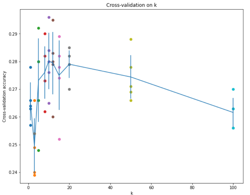
k가 10과 20 사이에 있을 때 accuracy가 높고 너무 높아지면 오히려 accuracy가 떨어졌다.
best_k = 10

classifier = KNearestNeighbor()
classifier.train(X_train, y_train)
y_test_pred = classifier.predict(X_test, k=best_k)

# Compute and display the accuracy
num_correct = np.sum(y_test_pred == y_test)
accuracy = float(num_correct) / num_test
print('Got %d / %d correct => accuracy: %f' % (num_correct, num_test, accuracy))
k=10 일 때 accuracy = 0.282000
여러 k를 대입했을 때, k=10일 때 accuracy가 가장 크게 나왔고 이 데이터셋에 대한 최적의 hyperparameter k는 10임을 확인했다.
'딥러닝 > cs231n' 카테고리의 다른 글
| 3장. Programming: Stochastic Gradient Descent (0) | 2021.03.05 |
|---|---|
| 4장. Neural Networks and Back Propagation (0) | 2021.03.05 |
| 3장. Multiclass Support Vector Machine : Programming (2) | 2021.02.27 |
| 3장. Loss Functions and Optimization (0) | 2021.02.18 |
| 2강. Image Classification (0) | 2021.02.16 |


