1. X_train과 y_train을 LinearSVM model로 train
LinearClassifier
LinearClassifier class에는 __init__(self), train(self, X, y, learning_rate=1e-3, reg=1e-5, num_iters=100, batch_size=200, verbose=False), predict(self, X), loss(self, X_batch, y_batch, reg) 함수가 있다.
또한, LinearSVM과 Softmax class는 LinearClassifier을 상속받아서 LinearClassifier의 함수들을 사용할 수 있고, 각각 loss 함수가 있다.
class LinearSVM(LinearClassifier):
    """ A subclass that uses the Multiclass SVM loss function """

    def loss(self, X_batch, y_batch, reg):
        return svm_loss_vectorized(self.W, X_batch, y_batch, reg)


class Softmax(LinearClassifier):
    """ A subclass that uses the Softmax + Cross-entropy loss function """

    def loss(self, X_batch, y_batch, reg):
        return softmax_loss_vectorized(self.W, X_batch, y_batch, reg)
class LinearClassifier(object):

    def __init__(self):
        self.W = None

    def train(self, X, y, learning_rate=1e-3, reg=1e-5, num_iters=100,
              batch_size=200, verbose=False):

        num_train, dim = X.shape
        num_classes = np.max(y) + 1 # assume y takes values 0...K-1 where K is number of classes
        if self.W is None:
            # lazily initialize W
            self.W = 0.001 * np.random.randn(dim, num_classes)

        loss_history = []
        for it in range(num_iters):
            X_batch = None
            y_batch = None

            mask = np.random.choice(num_train, batch_size, replace=True)
            X_batch = X[mask]
            y_batch = y[mask]
            X_batch=X_batch.reshape(batch_size, dim)
            y_batch=y_batch.reshape(batch_size,)

            # evaluate loss and gradient
            loss, grad = self.loss(X_batch, y_batch, reg)
            loss_history.append(loss)

            # perform parameter update

            self.W=self.W-learning_rate*grad

            if verbose and it % 100 == 0:
                print('iteration %d / %d: loss %f' % (it, num_iters, loss))

        return loss_history
num_train, dim, num_classes를 지정해준다.
LinearClassifier의 다른 함수로 계산을 하면서 W가 새로 update 되어 있을 수 있는데, 그렇지 않고 변수들에 대해 LinearClassifier을 처음 사용하는 경우 W를 새롭게 initialize 해준다.
batch size만큼 X, Y에서 random하게 꺼내서 X_batch, y_batch에 넣어주고, shape을 확실하게 해주기 위해 reshape 해준다.
실제로 코드를 돌릴 때, svm = LinearSVM() 또는 svm=Softmax()로 할당해주고 svm.train()을 계산하게 된다.
self.loss(X_batch, y_batch, reg)에서는, LinearSVM에서 정의한 loss 함수인 svm_loss_vectorized(self.W, X_batch, y_batch, reg)로 loss와 grad를 계산한다.
loss_history에 이렇게 계산한 loss를 추가하고, grad와 learning rate로 self.W를 update 한다.
from cs231n.classifiers import LinearSVM
svm = LinearSVM()
tic = time.time()
loss_hist = svm.train(X_train, y_train, learning_rate=1e-7, reg=2.5e4,
                      num_iters=1500, verbose=True)
toc = time.time()
print('That took %fs' % (toc - tic))
iteration 0 / 1500: loss 402.022700 iteration 100 / 1500: loss 238.979744 iteration 200 / 1500: loss 145.239858 iteration 300 / 1500: loss 88.584470 iteration 400 / 1500: loss 56.229948 iteration 500 / 1500: loss 35.774735 iteration 600 / 1500: loss 23.368881 iteration 700 / 1500: loss 16.003414 iteration 800 / 1500: loss 11.872691 iteration 900 / 1500: loss 9.099504 iteration 1000 / 1500: loss 7.115828 iteration 1100 / 1500: loss 6.266767 iteration 1200 / 1500: loss 5.577039 iteration 1300 / 1500: loss 5.600220 iteration 1400 / 1500: loss 5.811417 That took 9.116621s
svm=LinearSVM()으로 클래스를 불러와서 svm.train()으로 iter에 따라 W를 update 하면서 loss와 W를 update 한다.
plt.plot(loss_hist)
plt.xlabel('Iteration number')
plt.ylabel('Loss value')
plt.show()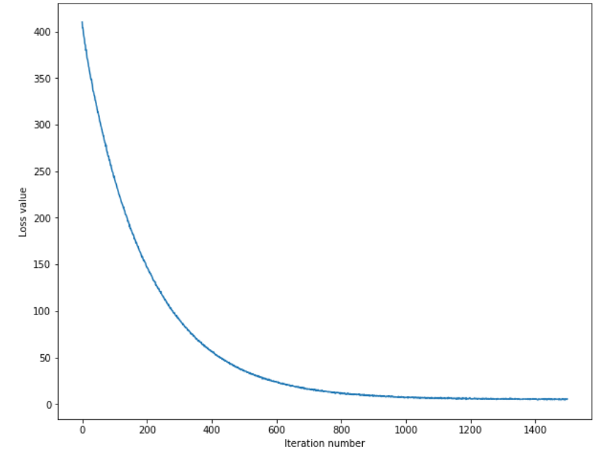
iter에 따라 Loss가 감소한다.
2. 학습한 model로 X_train, X_val 정확도 평가
y_train_pred = svm.predict(X_train)
print('training accuracy: %f' % (np.mean(y_train == y_train_pred), ))
y_val_pred = svm.predict(X_val)
print('validation accuracy: %f' % (np.mean(y_val == y_val_pred), ))
training accuracy: 0.385653 validation accuracy: 0.391000
3. 최적의 hyperparameter 찾기
results = {}
best_val = -1
best_svm = None
learning_rates = [1e-7, 5e-5]
regularization_strengths = [2e4, 2.5e4, 3e4, 3.5e4, 4e4, 4.5e4, 5e4, 6e4]
W = np.random.randn(3073, 10) * 0.0001
for lr in learning_rates:
for rg in regularization_strengths:
svm = LinearSVM()
loss_hist = svm.train(X_train, y_train, learning_rate=lr, reg=rg,
num_iters=1500, verbose=False)
y_train_pred = svm.predict(X_train)
train_accuracy = np.mean(y_train_pred == y_train)
y_val_pred = svm.predict(X_val)
val_accuracy = np.mean(y_val_pred == y_val)
results[(lr,rg)]=(train_accuracy,val_accuracy)
if val_accuracy > best_val:
best_val = val_accuracy
best_svm = svm
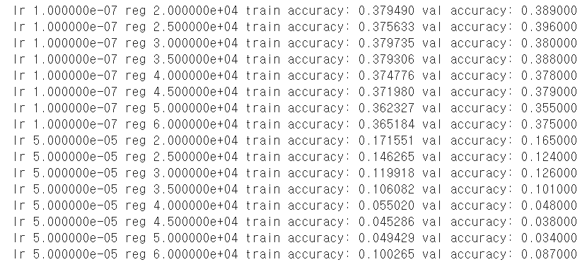
for lr, reg in sorted(results):
train_accuracy, val_accuracy = results[(lr, reg)]
print('lr %e reg %e train accuracy: %f val accuracy: %f' % (
lr, reg, train_accuracy, val_accuracy))
print('best validation accuracy achieved during cross-validation: %f' % best_val)class LinearClassifier(object):
def train(...):
....
def predict(self, X):
y_pred = np.zeros(X.shape[0])
score=np.dot(X,self.W)
y_pred = np.argmax(score,axis=1)
return y_pred다양한 learing rate와 reg로 X_train의 model 생성 후 train set, validation set의 accuracy를 평가 -> validation set의 accuracy가 가장 높은 model과 그 때의 hyperparameter을 선택한다.
svm = LinearSVM()으로 LinearSVM 클래스를 svm에 할당받았고, LinearSVM의 loss 함수, LinearClassifier의 train, predict, loss 함수를 사용할 수 있다.
loss_hist = svm.train(X_train, y_train, learning_rate=lr, reg=rg, num_iters=1500, verbose=False)
svm의 train 함수로 주어진 hyperparameter에 대해 train set을 학습시킨다. 이 결과 self.W는 1500번 iteration 이후 update 된 W이다.
y_train_pred = svm.predict(X_train)
predict에서 X와 self.W를 곱한 score에서 행별 최댓값을 y_pred에 담는다. 이 때 self.W는 __init__에서 self.W=None이 아니라, model train 후에 update 된 W이다.
train_accuracy = np.mean(y_train_pred == y_train)
y의 실제값과 예상값을 비교하여 accuracy를 평가한다. validation set에서도 동일하게 수행한다.
if validation_accuracy > best_val 구문에서 best_val과 best_svm을 update 한다.
best validation accuracy achieved during cross-validation: 0.396000
Training set, Validation set의 accuracy 시각화
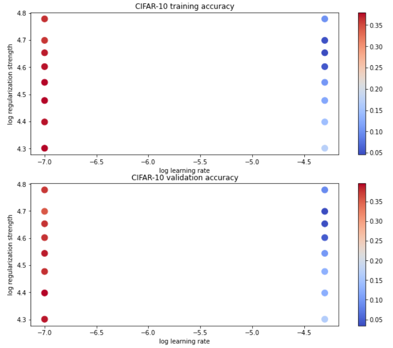
색이 진할 때 accuracy가 높은 것인데, log reg = 0.25~0.35 사이의 accuracy가 가장 높다.
4. Test set에 최적의 hyperparameter 적용 후 accuracy 평가
y_test_pred = best_svm.predict(X_test)
test_accuracy = np.mean(y_test == y_test_pred)
print('linear SVM on raw pixels final test set accuracy: %f' % test_accuracy)
linear SVM on raw pixels final test set accuracy: 0.365000
5. 각 class의 weigh 시각화
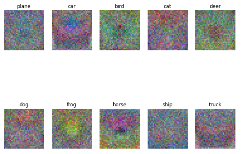
W를 4D로 reshape 하고 rescale 후 시각화하면 위와 같다. 각 class마다 사진이 시각화 결과와 비슷하면 높은 점수를 얻는다.
'딥러닝 > cs231n' 카테고리의 다른 글
| FullyConnected Nets: Programming 개요 (2) | 2021.03.13 |
|---|---|
| 5강. Convolutional Neural Network (4) | 2021.03.12 |
| 4장. Neural Networks and Back Propagation (0) | 2021.03.05 |
| 3장. Multiclass Support Vector Machine : Programming (2) | 2021.02.27 |
| 3장. Loss Functions and Optimization (0) | 2021.02.18 |


