1. Package 불러오기
목표
data.h5라는 data set에는 다양한 사진 데이터가 있고, 이것이 고양이인지(1) 아닌지(0) linear regression으로 분류하는 모델을 만들 것이다.
2. Problem Set에 대한 Overview
데이터 셋 확인
train_set_x_orig, train_set_y, test_set_x_orig, test_set_y, classes = load_dataset()
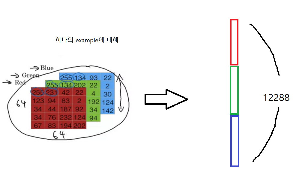
- train_set_x_org.shape (209, 64, 64, 3): 209개의 example을 가지고 있다. 하나의 example은 r,g,b의 채널을 가지고 각 채널에는 64*64의 array로 0~255개의 숫자가 표시된다. (하나의 example이 64*64짜리 array로 표시되는데, 각 unit은 r,g,b에 담긴 숫자들의 조합으로 색깔이 결정된다.)
- test_set_y.shape (1,209): 209개의 example에 대해 0또는 1의 값이 표시된다.
- test_set_x_orig.shape (50, 64, 64, 3): 50개의 example을 가지고 있고 train x data와 구조가 동일하다.
- test_set_y.shape (50,1) : 50개의 example을 가지고 있고 train y data와 구조가 동일하다.
example 확인하기
# Example of a picture
index = 25
plt.imshow(train_set_x_orig[index])
print ("y = " + str(train_set_y[:, index]) + ", it's a '" + classes[np.squeeze(train_set_y[:, index])].decode("utf-8") +  "' picture.")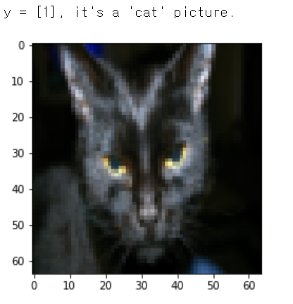
train_set에서 index = 25의 x data를 plt.imshow로 볼 수 있고, index=25의 y값이 1임을 확인했다.
c.f.) 참고사항 np.squeeze
np.squeeze(배열, axis=0,1,2)을 통해 지정된 축의 차원을 축소할 수 있음.
배열.shape=(1,3,1)일 때 axis=0이면 배열.shape=(3,1)
axis를 지정하지 않으면 기본값은 axis=0으로, 1차원 배열로 축소 한다.
data를 flatten 시켜주기
train_set_x_orig.shape은 (m_train, num_px, num_px, 3)의 꼴임. (왠만한 이미지 데이터는 이런 shape을 가진다.)
train_set_x_flatten = train_set_x_orig.reshape(train_set_x_orig.shape[0],-1).T
test_set_x_flatten = test_set_x_orig.reshape(test_set_x_orig.shape[0],-1).T
train_set_x shape: (209, 64, 64, 3) ===> train_set_x_flatten shape: (12288, 209)
test_set_x shape: (50, 64, 64, 3) ===> test_set_x_flatten shape: (12288, 50)
x train과 x test를 flatten 시켜줌. y는 변동 없음
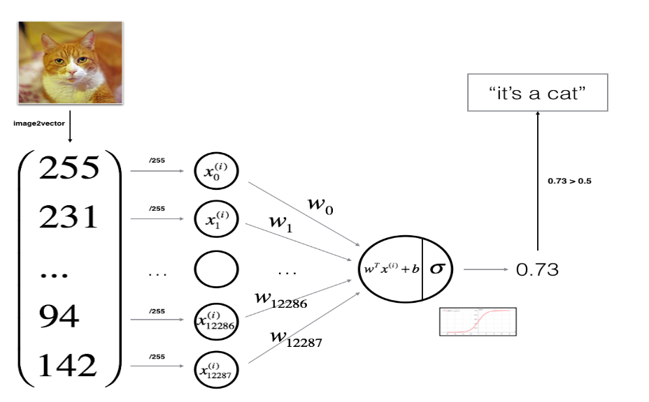
preprocessing - standardization
train_set_x = train_set_x_flatten/255
test_set_x = test_set_x_flatten/255
r,g,b에 해당하는 픽셀들은 0 ~ 255 사이의 정수만을 값으로 가지는데, standardization의 일환으로 모든 원소를 255로 나눠주면, 모델의 수렴이 빨라진다.
3. 알고리즘 학습에 대한 개요 확인
- model의 parameter(w,b)을 initialize 해준다.
- cost function을 minimize 하는 parameter을 학습한다.
- 학습된 parameter로 y 값을 test set에 대해 predict 한다.
- 결과를 분석하고 결론을 내린다.
4. 알고리즘 구현하기
- 모델의 구조를 파악하기
- 모델의 parameter initialize 하기
- iteration number로 loop 돌기
- forward propagation으로 당시 iter에 대한 loss 구하기
- backward propagation으로 당시 iter에 대한 w,b의 gradient 구하기
- gradient descent로 parameter을 update 하기
4.1 helper function 구현
def sigmoid(z):
	s = 1/(1+np.exp(-z))
 	return s
np.exp(x)를 이용하면 x안에 들어가는 것이 실수가 아닌 array라도 element-wise하게 계산된다.
4.2 initializing parameters
def initialize_with_zeros(dim):
    w = np.zeros((dim,1))
    b = 0

    assert(w.shape == (dim, 1))
    assert(isinstance(b, float) or isinstance(b, int))

    return w, b
dim은 x(i)의 feature의 수(nx)가 될 것이다. w는 1*nx짜리 벡터이고 element는 모두 0으로 채워주고 b는 0으로 해준다.
c.f.) assert()는 괄호 안이 참인지 확인해준다.
4.3 Forward and Backward Propagation
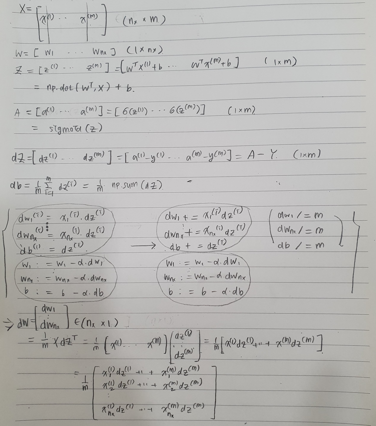

위처럼 X,W,b에 대해 A,cost를 구하는 과정이 forward propagation, dZ, db, dW를 구하는 과정이 backward propagation이다.
def propagate(w, b, X, Y):
m = X.shape[1]
A = sigmoid(np.dot(w.T,X)+b)
cost = (-1/m)*np.sum(Y*np.log(A)+(1-Y)*np.log(1-A))
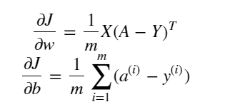
dw = (1/m)*np.dot(X,(A-Y).T)
db = (1/m)*np.sum(A-Y)
assert(dw.shape == w.shape)
assert(db.dtype == float)
cost = np.squeeze(cost)
assert(cost.shape == ())
grads = {"dw": dw, "db": db}
return grads, cost
4.4 Optimazation
각 iteration에서 구한 cost, grads(dw,db)로 gradient descent를 통해 w,b를 update 해야 한다.
def optimize(w, b, X, Y, num_iterations, learning_rate, print_cost = False):
    costs = []

    for i in range(num_iterations):
        grads, cost =  propagate(w, b, X, Y)

        dw = grads["dw"]
        db = grads["db"]

        w = w-learning_rate*dw
        b = b-learning_rate*db

        if i % 100 == 0:
            costs.append(cost)


        if print_cost and i % 100 == 0:
            print ("Cost after iteration %i: %f" %(i, cost))

    params = {"w": w,
              "b": b}

    grads = {"dw": dw,
             "db": db}

    return params, grads, costs
num_iteration의 횟수만큼 w,b를 갱신하는 과정을 반복할 것이다.
각 iteration에 대해 propagate()로 grads(w,b)와 cost를 구하고 w와 b를 갱신한다.
그리고 나중에 cost function이 잘 감소하고 있는 지 확인하기 위해 costs라는 리스트 안에 100회의 iteration마다 cost를 기록한다.
함수를 정의할 때 매개변수에 특정 값이 주어지면 그 값을 default로 사용한다.
여기선 print_cost=False 값을 default로 쓰는데, if print_cost (=True)이면 100회의 iteration마다 i에 따른 cost를 출력한다.
for문을 모두 돌고 나서 최종적인 변수들을 저장한다. params의 딕셔너리에 w와 b를, grads의 딕셔너리에 dw와 db를 저장한다.
+) predict
def predict(w, b, X):

    m = X.shape[1]
    Y_prediction = np.zeros((1,m))
    w = w.reshape(X.shape[0], 1)

    A = sigmoid(np.dot(w.T,X)+b)

    for i in range(A.shape[1]):
        Y_prediction[0,i]=(A[0,i]>=0.5)

    assert(Y_prediction.shape == (1, m))

    return Y_prediction
X에 대해 optimize()로 학습한 w,b로 y값을 예측한다. sigmoid(w(t)*x(i)+b)>=0.5면 y=1, <0.5면 y=0으로 예측한다.
Y = [y(1) ... y(m)], w = [w_1 ... x_nx].T, A = [a(1) ... a(m)]
a(i)의 값이 0.5보다 크면 i번째 Y의 prediction은 1이다.
4.5 하나의 모델로 합치기
def model(X_train, Y_train, X_test, Y_test, num_iterations = 2000, learning_rate = 0.5, print_cost = False):

    w, b = initialize_with_zeros(X_train.shape[0])

    parameters, grads, costs = optimize(w,b,X_train,Y_train,num_iterations,learning_rate, print_cost = False)

    w = parameters["w"]
    b = parameters["b"]

    Y_prediction_test = predict(w, b, X_test)
    Y_prediction_train = predict(w, b, X_train)


    # Print train/test Errors
    print("train accuracy: {} %".format(100 - np.mean(np.abs(Y_prediction_train - Y_train)) * 100))
    print("test accuracy: {} %".format(100 - np.mean(np.abs(Y_prediction_test - Y_test)) * 100))

    d = {"costs": costs, #optimize에서 나옴
         "Y_prediction_test": Y_prediction_test,  #prediction
         "Y_prediction_train" : Y_prediction_train,  #prediction
         "w" : w, #optimize에서 나옴
         "b" : b,#optimize에서 나옴
         "learning_rate" : learning_rate, #기본 설정값
         "num_iterations": num_iterations} #기본 설정값

    return d
w,b를 initialize_with_zeros로 initialize 해준다.
optimize로 현재의 w,b에 대해 forward, backward propagation을 해주고 costs와 grads(dw,db)를 구하고 그에 의해 갱신된 params(w,b)를 구한다.
최종 결정된 w,b로 test set과 train set을 predict로 예측한다.
(1/m)*Σ| ŷ(i)-y(i)| 으로 y와 ŷ을 비교하여 정확도를 구한다.
d에 이렇게 구한 costs, train set, test set의 예측한 y값, w, b 등을 return 한다.
결과
99.04%의 train set accuracy, 70.0 %의 test set accuracy를 보였다.
해석: train set에 overfitting 되었고 test set의 accuracy는 꽤 낮았다. (overfitting은 후에 regularization을 통해 조절할 것임)
Learning Curve를 Plotting
costs = np.squeeze(d['costs'])
plt.plot(costs)
plt.ylabel('cost')
plt.xlabel('iterations (per hundreds)')
plt.title("Learning rate =" + str(d["learning_rate"]))
plt.show()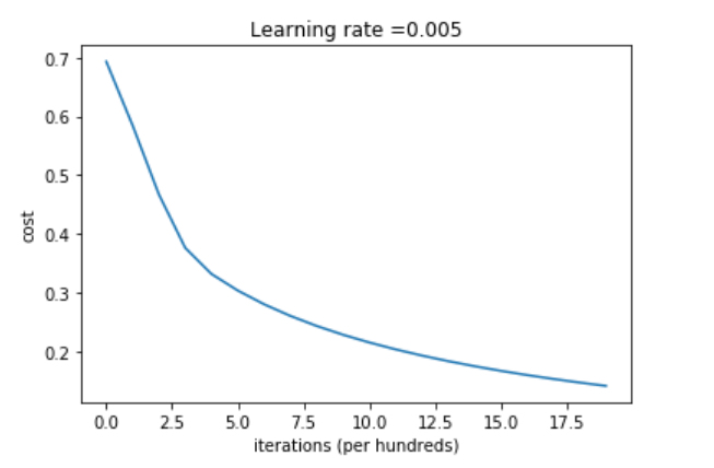
iteration에 따라 cost가 잘 감소하고 있음을 확인했다.
추가) Learning Rate의 선택
learning_rates = [0.01, 0.001, 0.0001]
models = {}
for i in learning_rates:
    print ("learning rate is: " + str(i))
    models[str(i)] = model(train_set_x, train_set_y, test_set_x, test_set_y, num_iterations = 1500, learning_rate = i, print_cost = False)

for i in learning_rates:
    plt.plot(np.squeeze(models[str(i)]["costs"]), label= str(models[str(i)]["learning_rate"]))

plt.ylabel('cost')
plt.xlabel('iterations (hundreds)')

legend = plt.legend(loc='upper center', shadow=True)
frame = legend.get_frame()
frame.set_facecolor('0.90')
plt.show()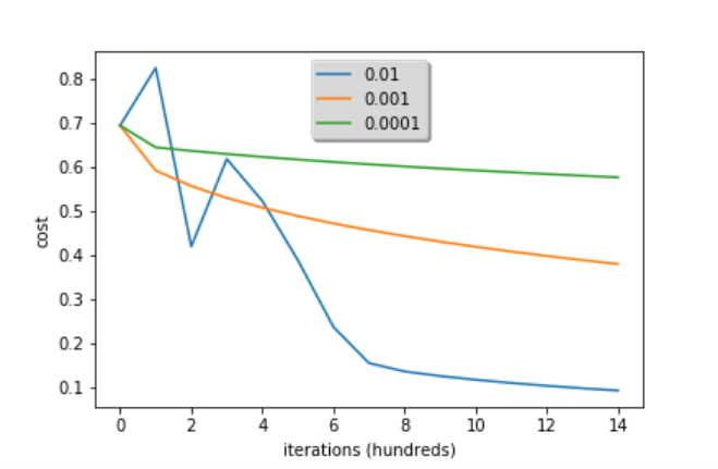
learning rate is: 0.01 train accuracy: 99.52153110047847 % test accuracy: 68.0 %
learning rate is: 0.001 train accuracy: 88.99521531100478 % test accuracy: 64.0 %
learning rate is: 0.0001 train accuracy: 68.42105263157895 % test accuracy: 36.0 %
learning rate = [0.01, 0.001, 0.0001]으로 모델을 학습한 결과 learning rate가 작아질 수록 적당한 w,b값을 찾아서 적절한 y값을 예측하는 데까지 시간이 너무 오래 걸리는 것을 알 수 있었다. train accuracy는 물론이고 test accuracy도 감소한다. 너무 크지도 작지도 않은 적당한 정도의 learning rate를 설정해야 한다.
'딥러닝 > DeepLearning.ai' 카테고리의 다른 글
| 3주차. Programming assignment (0) | 2021.02.05 |
|---|---|
| 3주차. Shallow Neural Network (0) | 2021.02.04 |
| 2주차. Vectorization (0) | 2021.02.03 |
| 2주차. Logistic Regression as a Neural Network (0) | 2021.02.02 |
| 1주차. Deep Learning introduction (0) | 2021.02.02 |


