1. packages
import numpy as np
import matplotlib.pyplot as plt
from testCases_v2 import *
import sklearn
import sklearn.datasets
import sklearn.linear_model
from planar_utils import plot_decision_boundary, sigmoid, load_planar_dataset, load_extra_datasets

%matplotlib inline

np.random.seed(1)
np.random.seed()로 결과값이 항상 동일하도록 설정했다.
2. dataset
X, Y = load_planar_dataset()
plt.scatter(X[0, :], X[1, :], c=Y, s=40, cmap=plt.cm.Spectral);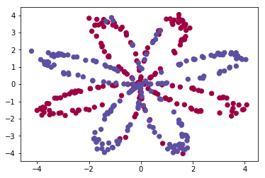
matplotlib의 scatter으로 산포도를 나타냈다. 가로축은 x1, 세로축은 x2이고 y=0이면 red, y=1이면 blue로 표시했다.
데이터의 shape 확인
X.shape: (2, 400)
Y.shape: (1,400)
총 400개의 example, X의 feature은 2개 (x1, x2)로 X는 example이 가로로 길게 늘어져 있는 형태이다. Y의 경우 0또는 1의 실수로만 이루어졌기 때문에 1개의 행만을 가진다.
3. Simple Logistic Regression
simple logistic regression이 이 데이터에 맞는 모델인지 확인해보겠다.
clf = sklearn.linear_model.LogisticRegressionCV();
clf.fit(X.T, Y.T);
sklearn의 linear_model package 패키지의 LogisticRegressionCV 함수는 logistic regression model 중 linear 한 decision boundary를 만들어주는 model이다. 선형의 단 하나의 decision boundary로 y=0과 1을 classify 할 수 있을까?
plot_decision_boundary(lambda x: clf.predict(x), X, Y)
plt.title("Logistic Regression")

# Print accuracy
LR_predictions = clf.predict(X.T)
print ('Accuracy of logistic regression: %d ' % float((np.dot(Y,LR_predictions) + np.dot(1-Y,1-LR_predictions))/float(Y.size)*100) +
       '% ' + "(percentage of correctly labelled datapoints)")
planar_utils 패키지에 plot_decision_boundary 함수가 내장되어 있고 이는 X,Y에 대해 predict 한 Y값으로 decision boundary를 나눠주는 함수이다.
clf 모델을 X에 적용하여 LR_predictions에 예상 y값을 넣어준다.
np.dot ( Y , LR_predictions ) : Y == 1 & LR_predictions == 1의 example 수
np.dot (1-Y , 1 - LR_predictions ) : Y==0 & LR_predictions == 0의 example 수
np.dot ( Y , LR_predictions ) + np.dot (1-Y , 1 - LR_predictions ) : 정답을 맞춘 example의 수, 이를 Y.size로 나눠서 accuracy를 계산함.
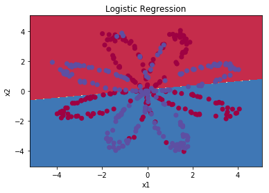
accuracy가 47%로 매우 낮았고 linear 한 decision boundary로 만든 logistic regerssion model로는 적절한 classification이 안되는 것을 알았다. Neural Network model을 생성해보자.
4. Neural Network Model
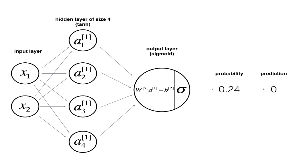
하나의 example이 x1,x2를 feature 가진다. 이 모델에서는 hidden layer 층을 하나로 해줄 것이고 이 층의 node를 4개로 설정했다. (a[1]_1 ~ a[1]_4) z에서 a로 활성화 함수로는 tanh function을 사용했다. 출력층에서는 활성화 함수를 sigmoid를 사용했다. (binary classification이기 때문) 이 때 출력값이 0.5 이상이면 y=1로, 0.5 미만이면 y=0으로 predict 할 것이다.
Neural Network를 만드는 방법
- network의 구조를 선택한다. (hidden layer의 수, hidden unit의 수)
- model의 parameter을 initialize 한다.
- loop
- forward propagation을 수행한다.
- loss를 계산한다.
- backward propagation을 수행한다.
- gradient descent로 parameter을 update 한다.
4.1 neural network의 구조 설정하기
- n_x: the size of the input layer
- n_h: the size of the hidden layer (set this to 4)
- n_y: the size of the output layer
def layer_sizes(X, Y):
    n_x = X.shape[0] # size of input layer
    n_h = 4
    n_y = Y.shape[0] # size of output layer

    return (n_x, n_h, n_y)
4.2 parameter initialize
# GRADED FUNCTION: initialize_parameters

def initialize_parameters(n_x, n_h, n_y):

    np.random.seed(2)

    W1 = np.random.randn(n_h,n_x)*0.01
    b1 = np.zeros((n_h,1))
    W2 = np.random.randn(n_y,n_h)*0.01
    b2 = np.zeros((n_y,1))

    assert (W1.shape == (n_h, n_x))
    assert (b1.shape == (n_h, 1))
    assert (W2.shape == (n_y, n_h))
    assert (b2.shape == (n_y, 1))

    parameters = {"W1": W1,
                  "b1": b1,
                  "W2": W2,
                  "b2": b2}

    return parameters
W1, W2는 다음 layer의 node 수 * 이전 layer의 node 수로 shape을 정해줘야 하고 symmetric breaking을 위해 random의 값들로 설정해줘야 한다. 그리고 *0.01을 해줘서 값을 작게 만들어준다. b1, b2는 실수인 0으로 설정한다.
assert로 shape이 적절한지 확인해주고 parameters이라는 딕셔너리 안에 넣어준다.
4.3 loop
def forward_propagation(X, parameters):

    # Retrieve each parameter from the dictionary "parameters"
    W1 = parameters["W1"]
    b1 = parameters["b1"]
    W2 = parameters["W2"]
    b2 = parameters["b2"]

    # Implement Forward Propagation to calculate A2 (probabilities)
    Z1 = np.dot(W1,X)+b1
    A1 = np.tanh(Z1)
    Z2 = np.dot(W2,A1)+b2
    A2 = sigmoid(Z2)

    assert(A2.shape == (1, X.shape[1]))

    cache = {"Z1": Z1,
             "A1": A1,
             "Z2": Z2,
             "A2": A2}

    return A2, cache
W1,b1,W2,b2를 받아서 Z1,A1,Z2,A2를 계산하고 cache 딕셔너리에 넣어준다.
def compute_cost(A2, Y, parameters):
m = Y.shape[1]
# Compute the cross-entropy cost
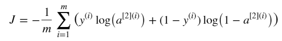
logprobs = np.multiply(np.log(A2),Y) + np.multiply(np.log(1-A2),1-Y)
cost = - np.sum(logprobs)/m
cost = float(np.squeeze(cost)) # makes sure cost is the dimension we expect.
# E.g., turns [[17]] into 17
assert(isinstance(cost, float))
return cost위에서 계산한 A2를 Y와 비교하여 cost를 계산해줘야 한다.
np.multiply(np.log(A2),Y))으로 Y=1일 때 np.log(A2) 값을 계산한다.
Y=[000111]으로 원소가 6개 있었으면 여기서 return 되는 값은 [000???]의 6개짜리 원소일 것이다.
np.multiply(np.log(1-A2),1-Y))으로 Y=0일 때 np.log(1-A2) 값을 계산한다.
Y=[000111]으로 원소가 6개 있었으면 여기서 return 되는 값은 [???000]의 6개짜리 원소일 것이다.
둘을 더하면 [??????]의 6개짜리 원소일 것이고 -np.sum()/m으로 원소들을 모두 합해주고 평균내준 뒤 마이너스를 해준다.
np.squeeze(cost)로 차원을 작게 만들어준다.
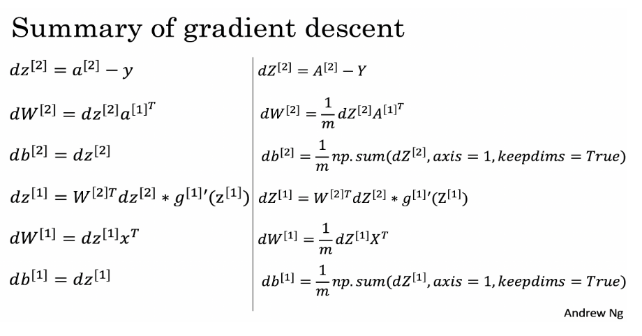
왼쪽은 backward propagation을 각 example별로, 오른쪽은 vectorization으로 처리하는 예시이다.
def backward_propagation(parameters, cache, X, Y):

    m = X.shape[1]

    # First, retrieve W1 and W2 from the dictionary "parameters".
    W1 = parameters['W1']
    W2 = parameters['W2']

    # Retrieve also A1 and A2 from dictionary "cache".
    A1 = cache["A1"]
    A2 = cache["A2"]

    # Backward propagation: calculate dW1, db1, dW2, db2.
    dZ2 = A2-Y
    dW2 = (1/m)*np.dot(dZ2,A1.T)
    db2 = (1/m)*np.sum(dZ2,axis=1,keepdims=True)
    dZ1 = np.dot(W2.T,dZ2)*(1-np.power(A1,2))
    dW1 = (1/m)*np.dot(dZ1,X.T)
    db1 = (1/m)*np.sum(dZ1,axis=1,keepdims=True)

    grads = {"dW1": dW1,
             "db1": db1,
             "dW2": dW2,
             "db2": db2}

    return grads
W1,W2,A1,A2 값을 받아온 뒤 dZ2,dW2,db2,dZ1,dW1,db1 값을 차례로 구한다.
참고로 dZ1 =np.dot(W2.T,dZ2)*(1-np.power(A1,2)) 으로 작성했는데, g(z)가 tanh일 때 g'(z)=1-{g(z)}^2이고, g(z)=A1이니까 g'(Z)=1-A1^2가 되기 때문에 뒷부분이 (1-np.power(A1,2)이 된 것이다.
update parameters
def update_parameters(parameters, grads, learning_rate = 1.2):

    # Retrieve each parameter from the dictionary "parameters"
    W1 = parameters['W1']
    b1 = parameters['b1']
    W2 = parameters['W2']
    b2 = parameters['b2']

    # Retrieve each gradient from the dictionary "grads"
    dW1 = grads['dW1']
    db1 = grads['db1']
    dW2 = grads['dW2']
    db2 = grads['db2']

    # Update rule for each parameter
    W1 = W1-learning_rate*dW1
    b1 = b1-learning_rate*db1
    W2 = W2-learning_rate*dW2
    b2 = b2-learning_rate*db2

    parameters = {"W1": W1,
                  "b1": b1,
                  "W2": W2,
                  "b2": b2}

    return parameters
parameters와 grads의 값을 모두 받고 W1,b1,W2,b2를 update 해준다.
4. Integrate model
def nn_model(X, Y, n_h, num_iterations = 10000, print_cost=False):
    np.random.seed(3)
    n_x = layer_sizes(X, Y)[0]
    n_y = layer_sizes(X, Y)[2]

    # Initialize parameters
    parameters = initialize_parameters(n_x, n_h, n_y)

    # Loop (gradient descent)

    for i in range(0, num_iterations):

        A2, cache = forward_propagation(X, parameters)
        cost = compute_cost(A2, Y, parameters)
        grads = backward_propagation(parameters, cache, X, Y)
        parameters =  update_parameters(parameters, grads)

        # Print the cost every 1000 iterations
        if print_cost and i % 1000 == 0:
            print ("Cost after iteration %i: %f" %(i, cost))

    return parameters
nx,ny를 설정하고 parameter을 initialize 한 후 iteration 횟수마다 forward propagation, cost 계산 backward propagation, parameter update를 수행한다.
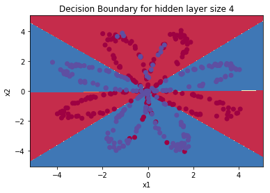
parameters = nn_model(X, Y, n_h = 4, num_iterations = 10000, print_cost=True)

# Plot the decision boundary
plot_decision_boundary(lambda x: predict(parameters, x.T), X, Y)
plt.title("Decision Boundary for hidden layer size " + str(4))
Cost after iteration 0: 0.693048
Cost after iteration 1000: 0.288083
Cost after iteration 2000: 0.254385
Cost after iteration 3000: 0.233864
Cost after iteration 4000: 0.226792
Cost after iteration 5000: 0.222644
Cost after iteration 6000: 0.219731
Cost after iteration 7000: 0.217504
Cost after iteration 8000: 0.219471
Cost after iteration 9000: 0.218612
iteration이 반복될수록 cost가 줄어들었고 plot에서 확인해도 decision boundary가 잘 형성이 되었다.
predictions = predict(parameters, X)
print ('Accuracy: %d' % float((np.dot(Y,predictions.T) + np.dot(1-Y,1-predictions.T))/float(Y.size)*100) + '%')
accuracy는 90%로 높은 편에 속했다.
'딥러닝 > DeepLearning.ai' 카테고리의 다른 글
| 4주차. Programming: Building deep neural network (0) | 2021.02.07 |
|---|---|
| 4주차. Deep Neural Networks (0) | 2021.02.07 |
| 3주차. Shallow Neural Network (0) | 2021.02.04 |
| 2주차. Programming: Logistic Regression with Neural Network mindset (0) | 2021.02.03 |
| 2주차. Vectorization (0) | 2021.02.03 |


