1. packages
import time
import numpy as np
import h5py
import matplotlib.pyplot as plt
import scipy
from PIL import Image
from scipy import ndimage
from dnn_app_utils_v3 import *

%matplotlib inline
plt.rcParams['figure.figsize'] = (5.0, 4.0) # set default size of plots
plt.rcParams['image.interpolation'] = 'nearest'
plt.rcParams['image.cmap'] = 'gray'

%load_ext autoreload
%autoreload 2

np.random.seed(1)
2. Dataset
train_x_orig, train_y, test_x_orig, test_y, classes = load_data()logistic regression as a neural network에서의 동일한 dataset을 사용할 것이다. y에는 cat인지(1) cat이 아닌지(0)의 정보가 있고, x에는 하나의 example이 (num_px, num_px, 3)의 구조를 가지고 있다. 이 데이터셋에서는 num_px = 64로, R,G,B channel이 0~255 사이의 값을 가진다.
Number of training examples: 209
Number of testing examples: 50
Each image is of size: (64, 64, 3)
train_x_orig shape: (209, 64, 64, 3)
train_y shape: (1, 209)
test_x_orig shape: (50, 64, 64, 3)
test_y shape: (1, 50)
다음으로는, 이미지 데이터(x train, x test)를 (209, 64, 64, 3)이 아닌 (64*64*3, 209) 즉, (12288, 209)로 각 example에 대한 RGB 값을 길게 늘여서 벡터 형태로 만들 것이고 이 example들을 가로로 죽 쌓는 reshape을 해주고 standardization을 해 줄 것이다.
# Reshape the training and test examples
train_x_flatten = train_x_orig.reshape(train_x_orig.shape[0], -1).T   # The "-1" makes reshape flatten the remaining dimensions
test_x_flatten = test_x_orig.reshape(test_x_orig.shape[0], -1).T

# Standardize data to have feature values between 0 and 1.
train_x = train_x_flatten/255.
test_x = test_x_flatten/255.

print ("train_x's shape: " + str(train_x.shape))
print ("test_x's shape: " + str(test_x.shape))
이렇게 train_x_flatten, test_x_flatten에 reshape 된 데이터셋을 넣어주고 모든 원소를 255로 나누는 standardization을 거쳐 최종적으로 train_x, test_x의 형태로 만들어준다.
train_x's shape: (12288, 209)
test_x's shape: (12288, 50)
3. Architecture of your model
이러한 데이터셋을 2 layer neural network와 deep neural network로 모델을 만들어서 두 모델을 평가할 것이다.
- A 2-layer neural network
- An L-layer deep neural network
3.1 2-layer neural network
주어진 x에 대해 linear relu로 a[1]를 계산하고 linear sigmoid로 a[2]를 계산하여 y=0 또는 1을 예측하는 2층짜리 neural network를 만들 수 있다.
W[1],b[1],W[2],b[2]의 parameter가 필요하다.
3.2 L-layer deep neural network
x (12288,1)에 대해 linear relu로 z[1],a[1], ... , z[l-1],a[l-1]을 계산하고 linear sigmoid로 z[l],a[l]을 계산하여 y=0 또는 1을 예측하는 L개의 층을 가진 neural network를 만들 수 있다.
각 층마다 W[l],b[l]의 parameter가 필요할 것이다.
3.3 General methodology
- parameter를 초기화한다.
- num_iteration 만큼 loop를 돈다.
- forward propagation
- cost function을 계산
- back propagation
- parameter을 update
- trained parameter로 label을 predict
4. Two-layer neural network
[LINEAR -> RELU] -> [LINEAR -> SIGMOID]
layer의 node 수를 다음과 같이 정했다.
n_x = 12288     # num_px * num_px * 3
n_h = 7
n_y = 1
layers_dims = (n_x, n_h, n_y)
# GRADED FUNCTION: two_layer_model

def two_layer_model(X, Y, layers_dims, learning_rate = 0.0075, num_iterations = 3000, print_cost=False):

    np.random.seed(1)
    grads = {}
    costs = []                              # to keep track of the cost
    m = X.shape[1]                           # number of examples
    (n_x, n_h, n_y) = layers_dims

    # Initialize parameters dictionary, by calling one of the functions you'd previously implemented
    parameters = initialize_parameters(n_x, n_h, n_y)

    # Get W1, b1, W2 and b2 from the dictionary parameters.
    W1 = parameters["W1"]
    b1 = parameters["b1"]
    W2 = parameters["W2"]
    b2 = parameters["b2"]

    # Loop (gradient descent)

    for i in range(0, num_iterations):

        # Forward propagation: LINEAR -> RELU -> LINEAR -> SIGMOID. Inputs: "X, W1, b1, W2, b2". Output: "A1, cache1, A2, cache2".
        A1, cache1 = linear_activation_forward(X, W1, b1, activation="relu")
        A2, cache2 = linear_activation_forward(A1, W2, b2, activation="sigmoid")

        # Compute cost
        cost = compute_cost(A2, Y)

        # Initializing backward propagation
        dA2 = - (np.divide(Y, A2) - np.divide(1 - Y, 1 - A2))

        # Backward propagation. Inputs: "dA2, cache2, cache1". Outputs: "dA1, dW2, db2; also dA0 (not used), dW1, db1".
        dA1, dW2, db2 = linear_activation_backward(dA2, cache2, activation="sigmoid")
        dA0, dW1, db1 = linear_activation_backward(dA1, cache1, activation="relu")

        # Set grads['dWl'] to dW1, grads['db1'] to db1, grads['dW2'] to dW2, grads['db2'] to db2
        grads['dW1'] = dW1
        grads['db1'] = db1
        grads['dW2'] = dW2
        grads['db2'] = db2

        # Update parameters.
        parameters = update_parameters(parameters, grads, learning_rate)

        # Retrieve W1, b1, W2, b2 from parameters
        W1 = parameters["W1"]
        b1 = parameters["b1"]
        W2 = parameters["W2"]
        b2 = parameters["b2"]

        # Print the cost every 100 training example
        if print_cost and i % 100 == 0:
            print("Cost after iteration {}: {}".format(i, np.squeeze(cost)))
        if print_cost and i % 100 == 0:
            costs.append(cost)

    # plot the cost

    plt.plot(np.squeeze(costs))
    plt.ylabel('cost')
    plt.xlabel('iterations (per hundreds)')
    plt.title("Learning rate =" + str(learning_rate))
    plt.show()

    return parameters
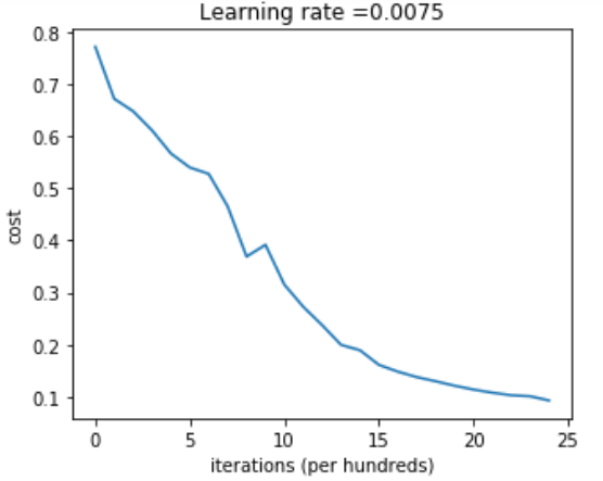
parameters = two_layer_model(train_x, train_y, layers_dims = (n_x, n_h, n_y), num_iterations = 2500, print_cost=True)
Cost after iteration 0: 0.6930497356599888
Cost after iteration 100: 0.6464320953428849
Cost after iteration 200: 0.6325140647912677
...
Cost after iteration 2400: 0.048554785628770115
iteration 할 수록 cost가 계속 줄어드는 것을 확인할 수 있다.
predictions_train = predict(train_x, train_y, parameters)Accuracy: 1.0
predictions_test = predict(test_x, test_y, parameters)Accuracy: 0.72
test set에서는 early stopping을 하면 모델의 성능이 더 좋아진다: 과적합이 되기 전에 iteration을 멈추는 것. 초기에 2400회 iteration을 설정했으나 1500회 때 early stopping을 할 수 있음.
logistic regression implementation (Accuracy: 70%)보다 성능이 좋아졌다.
5. L-layer neural network
[LINEAR -> RELU] × (L-1) -> [LINEAR -> SIGMOID]
layer의 node 수를 다음과 같이 설정했다.
layers_dims = [12288, 20, 7, 5, 1] # 4-layer model
def L_layer_model(X, Y, layers_dims, learning_rate = 0.0075, num_iterations = 3000, print_cost=False):#lr was 0.009

    np.random.seed(1)
    costs = []                         # keep track of cost

    # Parameters initialization. (≈ 1 line of code)
    parameters = initialize_parameters_deep(layers_dims)

    # Loop (gradient descent)
    for i in range(0, num_iterations):

        # Forward propagation: [LINEAR -> RELU]*(L-1) -> LINEAR -> SIGMOID.
        AL, caches =  L_model_forward(X, parameters)

        # Compute cost.
        cost = compute_cost(AL, Y)

        # Backward propagation.
        grads = L_model_backward(AL, Y, caches)

        # Update parameters.
        parameters = update_parameters(parameters, grads, learning_rate)

        # Print the cost every 100 training example
        if print_cost and i % 100 == 0:
            print ("Cost after iteration %i: %f" %(i, cost))
        if print_cost and i % 100 == 0:
            costs.append(cost)

    # plot the cost
    plt.plot(np.squeeze(costs))
    plt.ylabel('cost')
    plt.xlabel('iterations (per hundreds)')
    plt.title("Learning rate =" + str(learning_rate))
    plt.show()

    return parameters
parameters = L_layer_model(train_x, train_y, layers_dims, num_iterations = 2500, print_cost = True)Cost after iteration 0: 0.771749
Cost after iteration 100: 0.672053
Cost after iteration 200: 0.648263
...
Cost after iteration 2400: 0.092878
iteration에 따라 cost가 줄어들고 있는 것을 확인할 수 있다.
pred_train = predict(train_x, train_y, parameters)Accuracy: 0.985645933014
pred_test = predict(test_x, test_y, parameters)Accuracy: 0.8
2 layer neural network (Accuracy: 72%)에 비해 정확도가 증가했다.
6. Result Analysis
print_mislabeled_images(classes, test_x, test_y, pred_test)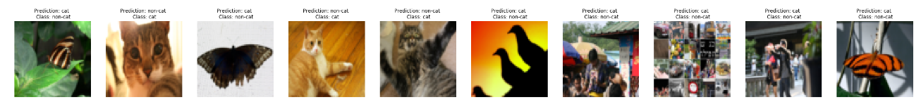
A few types of images the model tends to do poorly on include:
- Cat body in an unusual position
- Cat appears against a background of a similar color
- Unusual cat color and species
- Camera Angle
- Brightness of the picture
- Scale variation (cat is very large or small in image)
'딥러닝 > DeepLearning.ai' 카테고리의 다른 글
| 4주차. Programming: Building deep neural network (0) | 2021.02.07 |
|---|---|
| 4주차. Deep Neural Networks (0) | 2021.02.07 |
| 3주차. Programming assignment (0) | 2021.02.05 |
| 3주차. Shallow Neural Network (0) | 2021.02.04 |
| 2주차. Programming: Logistic Regression with Neural Network mindset (0) | 2021.02.03 |


