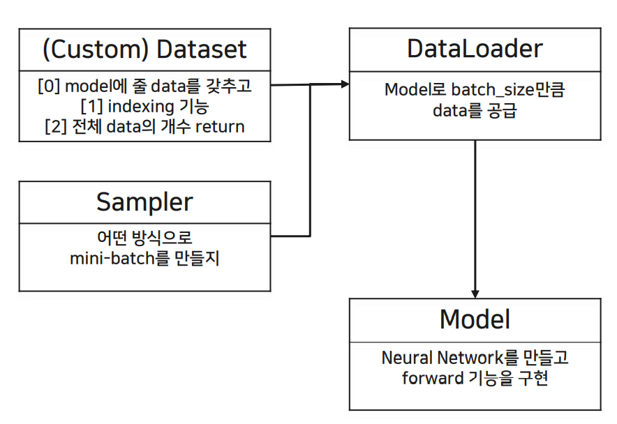
<Pytorch에서 구현해야 할 class>
(1) Custom Dataset: dataset을 model이 인식 가능한 형태로 custom하고, data의 index이 가능하도록 하고, 전체 data의 개수를 return하는 함수도 구현한다.
(2) Sampler: dataset을 model에 적용할 때 mini-batch 형태로 넘겨줄 것인데, 전체 dataset에서 batch를 어떤 식으로 만들 지 정해줌, ramdom sampler 등
(3) Data Loader: data를 batch_size만큼 model로 load 해주는 역할
(4) Model: neural network를 만들고 forward propagation 과정을 수행
<Pytorch 진행 순서>
0. Data upload
1. Data Load -1) Custom Dataset: FashionDataset(init, getitem, len) 클래스에서 구현
-2) Sampler
-3) Data Loader
2. Build Model - FashionCNN 클래스(init, forward)에서 구현
3. Train & Validation
패키지, 데이터 불러오기
import numpy as np
import pandas as pd
import matplotlib.pyplot as plt
import gzip
from tqdm import tqdm

import torch
import torch.nn as nn
#from torch.autograd import Variable

#import torchvision
import torchvision.transforms as transforms
from torch.utils.data import Dataset, DataLoader
from sklearn.metrics import confusion_matrix
난수 설정
def set_seed(RANDOM_SEED=42):
    torch.manual_seed(RANDOM_SEED)
    np.random.seed(RANDOM_SEED)
    torch.cuda.manual_seed(RANDOM_SEED)
    torch.cuda.manual_seed_all(RANDOM_SEED) # if use multi-GPU
    torch.backends.cudnn.deterministic = True
    torch.backends.cudnn.benchmark = False
    import random
    random.seed(RANDOM_SEED)

set_seed()
0. Data Upload
!git clone https://github.com/yeonseok-jeong-cm/yeonseok_fashion_mnist

with gzip.open('./yeonseok_fashion_mnist/fashion-mnist_train.gz') as f:
    train_csv = pd.read_csv(f)

with gzip.open('./yeonseok_fashion_mnist/fashion-mnist_test.gz') as f:
    test_csv = pd.read_csv(f)

train_csv
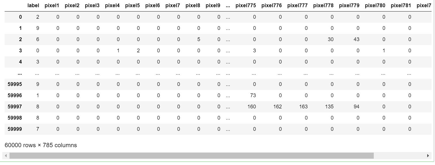
train_csv: 60000 * 785의 shape을 가지고, 0번째 열은 정답값에 해당한다.
test_csv: 10000 * 785
1. DataLoader
1) Custom Dataset
class FashionDataset(torch.utils.data.Dataset):

    def __init__(self, data, transform = None):
        self.fashion_MNIST = list(data.values)
        self.transform = transform

        label = []
        image = []

        # 1-0> csv data를 row 하나씩 list에 저장
        for i in self.fashion_MNIST:
            label.append(i[0])
            image.append(i[1:])
        # 1-1> numpy dataset 생성 (3d-array가 모여 4d-array 형태)
        self.labels = np.asarray(label)
        self.images = np.asarray(image).reshape(-1, 28, 28, 1).astype('float32')

    def __getitem__(self, index):
        # 2-2> indexing 기능을 구현
        label = self.labels[index]
        image = self.images[index]

        # 1-2> 추후 ToTensor로 numpy dataset을 Tensor dataset으로 변환
        if self.transform is not None:
            image = self.transform(image)

        return image, label

    def __len__(self):
        # 2-3> data 개수를 return
        return len(self.images)
내부 데이터를 tensor 형태로 만든다.
(하나의 example에 대하여) [ csv(1D) -> numpy(3D: W, H, C) ->(ToTensor) tensor ]
①__init__: 생성자
train_csv를 data로 받아와서 data의 value를 fashion_MNIST의 list로 받는다.
각 example에 대해 첫번째 열은 label로, 나머지 열은 image로 넣는다. 이때까진 label: 1D list, image: 2D list이다.
label과 image를 asarray()로 array로 바꿔준다. image는 reshape으로 (N, W, H, C)의 구조를 갖도록 만들어서 label: 1D array, image: 4D array가 되도록 한다.
② __getitem__: indexing 기능 구현
index를 input으로 받아서 image와 label의 index를 출력할 수 있도록 해준다.
③ __len__ : data의 개수 return
len으로 data의 총 개수를 알려준다.
=> ①~③으로 pytorch에서 사용할 수 있는 data 형태가 되었다.
train_set = FashionDataset(train_csv, transform=transforms.Compose([transforms.ToTensor()]))
test_set = FashionDataset(test_csv, transform=transforms.Compose([transforms.ToTensor()]))
array 형태로 바꾼 data를 ToTensor()로 tensor 형태로 바꿔서 train_set, test_set을 만들었다.
train_set.images.shape
(60000, 28, 28, 1) train_set은 4D shape의 tensor이 되었다.
2) Sampler
dataset에서 mini-batch만큼 추출할 때 (비복원 추출) 어떠한 규칙으로 추출할지 정하는 과정
mini-batch(표본) 내부 구성이 다양할수록 전체 dataset(모집단)를 잘 대표하기 때문에 주로 RandomSampler를 사용한다.
from torch.utils.data import RandomSampler

train_random_sampler = RandomSampler(train_set)
test_random_sampler = RandomSampler(test_set)
RandomSampler 클래스를 가져와서 train_set, test_set에 적용한다.
3) DataLoader
- 만들어진 dataset을
- batch_size만큼 (필요한 만큼)
- sampler라는 규칙으로 data를 추출해주는 class
BATCH_SIZE = 32

train_loader = DataLoader(train_set, batch_size=BATCH_SIZE, sampler=train_random_sampler)
test_loader = DataLoader(test_set, batch_size=BATCH_SIZE, sampler=test_random_sampler)
dataset(train_set, test_set)을 BATCH_SIZE만큼 train/test_random_sampler 규칙으로 load 해준다.
+) DataLoader의 내부 확인하기
train_iterator = iter(train_loader)
dir(train_iterator)
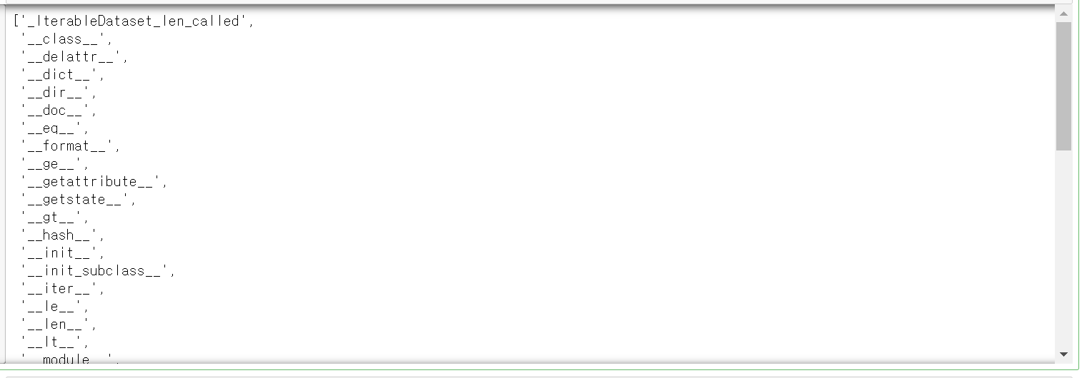
dir(iter(객체))로 객체 안의 메서드들을 확인할 수 있다.
'next' 객체가 있음을 확인했고, a1 = next(train_iterator)으로 객체의 shape을 확인할 수 있다.
a1[0].shape
# torch.Size([32, 1, 28, 28])
a1[1].shape
# torch.Size([32])
+) label mapping
def output_label(label):
    output_mapping = {
                 0: "T-shirt/Top",
                 1: "Trouser",
                 2: "Pullover",
                 3: "Dress",
                 4: "Coat",
                 5: "Sandal",
                 6: "Shirt",
                 7: "Sneaker",
                 8: "Bag",
                 9: "Ankle Boot"
                 }
    input = (label.item() if type(label) == torch.Tensor else label)
    return output_mapping[input]
각 class가 어떻게 mapping 되었는 지를 나타냄
2. Build the Model
class FashionCNN(nn.Module):

    def __init__(self):
        super(FashionCNN, self).__init__()

        self.layer1 = nn.Sequential(
            nn.Conv2d(in_channels=1, out_channels=32, kernel_size=3, padding=1),
            nn.BatchNorm2d(32),
            nn.ReLU(),
            nn.MaxPool2d(kernel_size=2, stride=2)
        )

        self.layer2 = nn.Sequential(
            nn.Conv2d(in_channels=32, out_channels=64, kernel_size=3),
            nn.BatchNorm2d(64),
            nn.ReLU(),
            nn.MaxPool2d(2)
        )

        self.fc1 = nn.Linear(in_features=64*6*6, out_features=600)
        self.drop = nn.Dropout2d(0.25)
        self.fc2 = nn.Linear(in_features=600, out_features=120)
        self.fc3 = nn.Linear(in_features=120, out_features=10)

    def forward(self, x):
        out = self.layer1(x)
        out = self.layer2(out)
        out = out.view(out.size(0), -1)
        out = self.fc1(out)
        out = self.drop(out)
        out = self.fc2(out)
        out = self.fc3(out)

        return out
FashionCNN 클래스로 model 안에 __init__, forward 함수를 만들 것이고 nn.Module을 상속받아서 neural network를 만들 것이다.
① __init__: 네트워크 내부에서 사용할 구조를 만든다.
Keras에서 사용하던 Sequential 방법으로 layer을 쌓을 수 있고 pytorch에서도 이를 이용할 수 있다.
[layer1 -> layer2 -> fc1 -> drop -> fc2 -> fc3]
layer 1을 sequential 방법으로 4개의 layer (CNN, batch normalization, activation, maxpooling)을 쌓을 것이다
fc1: tensorflow에서 dense를 의미함, fully-connected layer
fc1 -> fc2 -> fc3를 거치면서 in ~ out일 때 데이터 형태를 지정한다.
② forward: forward propagation 구현
후에 fully connected layer인 fc1~fc3을 거치기 위해 view로 3D -> 1D reshape을 해준다.
| cf> Train vs validation(Test) Train : forward propagation, compute loss, backpropagation, gradient descent Test : forward propagation -> FashionCNN으로 model을 만드는데, train set의 model 학습 과정에만 FashionCNN이 필요해서 forward 과정까지만 넣어줄 것이다. |
3. Train & Validation
device = torch.device("cuda:0" if torch.cuda.is_available() else "cpu")
device
# device(type='cpu')
cpu 혹은 gpu를 확인한다.
model = FashionCNN()
model.to(device)
--- model을 정의하고 device에 model을 올리는 과정

LEARNING_RATE = 0.001
EPOCHS = 3
BATCH_SIZE = 2**5
hyperparameter 설정
error = nn.CrossEntropyLoss()
optimizer = torch.optim.Adam(model.parameters(), lr=LEARNING_RATE)
total_batch = len(train_loader)
print(model)
train을 하기 위해 loss와 optimizer 연산이 필요하다.
Cross Entropy Loss로 loss를 정의했고, gradient descent인 optimzer은 Adam 방식으로 할 것이다.
1) Train
## 1) Train

for epoch in range(EPOCHS):
    print('\n'+'*'*50)
    print(f'Epoch {epoch+1}')
    avg_cost = 0
    model.train() # train mode
    for X, Y in tqdm(train_loader): # batch_size 단위로 꺼내온다.
        # 0> 연산하고자 하는 Tensor를 사용하는 device에 올려준다.
        X, Y = X.to(device), Y.to(device)
        # 2> forward propagation
        hypothesis = model(X)
        # 3> compute loss(cost) function
        cost = error(hypothesis, Y)
        ## backpropagation 단계 전에, Optimizer 객체를 사용하여 (모델의 학습 가능한 가중치인) 갱신할 변수들에 대한 모든 변화도를 0으로 만듭니다.
        ## 이렇게 하는 이유는 기본적으로 .backward()를 호출할 때마다 변화도가 버퍼(buffer)에 (덮어쓰지 않고) 누적되기 때문입니다.
        optimizer.zero_grad()
        # 4> backward propagation
        cost.backward()
        # 5> gradient descent
        optimizer.step()

        avg_cost += cost / total_batch

print('[Epoch: %d] train loss = %0.9f' % (epoch + 1, avg_cost))model.train(): train 과정임을 명시
train set에서 batch size만큼 mini batch를 돌릴 것이고 avg_cost에 loss를 저장할 것이다.
data loader인 train loader에서 batch size만큼 X, Y를 꺼내오고 to(device)로, device에 data를 올린다. (device에 model과 data를 올려야 한다.)
hypothesis=model(X)로 forward propagation을 수행한다.
위에서 정의한 error()로 cross entropy loss를 계산한다.
optimizer을 하기 전에 zero_grad()로 초기화 해준다.
.backward()로 back prop을 수행하고,
.step()으로 grad descent를 한다.
2) Validation
    correct = 0
    total = 0
    with torch.no_grad(): # Neural Network 연산 중에 gradient를 저장할 필요가 없으므로
        model.eval() # validation mode
        for X_val, Y_val in tqdm(test_loader):
            # 0> 연산하고자 하는 Tensor를 사용하는 device에 올려준다.
            X_val, Y_val = X_val.to(device), Y_val.to(device)
            # 2> forward propagation
            hypothesis = model(X_val)
            # calculate accuracy
            _, predicted = torch.max(hypothesis, 1)
            total += Y_val.size(0)
            correct += (predicted == Y_val).sum().item()

    print('[Epoch: %d] val accuracy = %0.2f %%' % (epoch + 1, 100. * float(correct / total)))
validation에서는 grad를 계산할 필요가 없어서 torch.no_grad()를 해준다.
model.eval(): validation 과정임을 명시
test_loader에서 batch_size만큼 X_val, Y_val을 꺼내오고, 이 데이터를 device에 올려준다.
forward propagation으로 Y_val을 예측한다.
Y_val의 예측값과 실제값 사이 accuracy를 구해야 한다.
torch.max()로 hypothesis에서 score이 가장 높게 나온 class를 predicted에 저장하고,
predicted와 Y_val 사이 정확도를 correct 안에 계산한다.
'머신러닝 > 분석 base' 카테고리의 다른 글
| Keras, TensorFlow (0) | 2021.03.04 |
|---|---|
| Resnet (0) | 2021.02.23 |
| Boosting & Adaboost (0) | 2021.02.09 |
| Bagging & Random Forest : Programming (0) | 2021.02.09 |
| Bagging & Random Forest (0) | 2021.02.09 |


