import tensorflow as tf
from tensorflow import keras
!pip install tensorflow로 tensorflow를 깔고, 위처럼 import를 해준다.
tensorflow로 iris를 분류하는 모델을 만들겠다.
from sklearn.datasets import load_iris
iris = load_iris()
X,y_ori = iris.data, iris.target
iris.target으로 받은 y_ori는 0, 1, 2로 구분되어 있다. 0, 1, 2는 명목형 변수로 대소관계가 없기 때문에 이를 one hot encoding으로 만들어주겠다.
from tensorflow.keras.utils import to_categorical
y = to_categorical(y_ori,3)
y는 [1,0,0], [0,1,0], ...으로 one hot encoding 되었다.
from sklearn.model_selection import train_test_split
X_train,X_test,y_train,y_test = train_test_split(X,y,random_state=0, test_size=0.3)
train_test_split으로 train, test set을 나눠주었다.
from keras.models import Sequential
from keras.layers import Dense

model = Sequential()
model.add(Dense(units=8, input_dim=4, kernel_initializer='uniform', activation='relu'))
model.add(Dense(units=3, activation='softmax'))
keras는 Sequential()로 layer를 순차적으로 쌓을 수 있다. model에 Sequential을 부여하고, add(Dense(...))로 순차적으로 층을 쌓아 준다. units=8은 해당 layer의 노드의 개수로, 임의로 설정해 준 값이다. input_dim = 4는 X에 4개의 feature이 input으로 들어간다는 의미이다. activation function은 relu로 설정했다.
다음으로, model.add(Dense(...))으로 마지막 층을 쌓아 준다. 마지막 층은 출력 층으로, 총 3가지의 class를 분류하는 모델이므로 units = 3으로 설정해야 한다. 또한, 출력층이고 multiclass를 분류하는 모델이므로 activation function은 softmax로 설정한다. binary class를 분류할 땐 relu로 해주어도 무방하다.
사실상 input layer와 output layer밖에 없는, 가장 간단한 형태의 모델이다.
model.compile(loss='categorical_crossentropy', optimizer='adam', metrics=['accuracy'])model을 쌓아주었으므로 model의 학습 과정에서의 변수들을 설정 해준다. multiclass 분류이므로 loss function은 categorical cross entropy로 설정했다. optimizer는 가장 성능이 좋다고 알려진(물론 데이터셋에 대해 성능에 차이가 있을 수 있다) adam으로 설정했다. metrics는 평가 지표로, accuracy를 설정했다.
model.summary()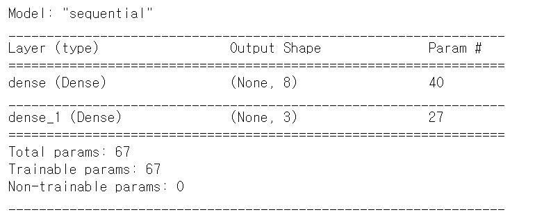
model.summary()로 layer의 구조를 확인할 수 있다.
hist = model.train(X_train,y_train, epochs = 100, batch_size=1, verbose = 2)train set으로 model을 학습시켰다. verbose는 학습 경과를 출력하는 옵션으로, verbose = 0은 출력하지 않는 것, verbose =1은 진행 막대와 함께 경과 출력, verbose = 2는 경과만 출력이다.
학습한 모델을 변수에 담아주면, 변수에서 accuracy와 loss의 경과를 따로 출력할 수 있다.
hist.history['accuracy'] # hist.history['loss']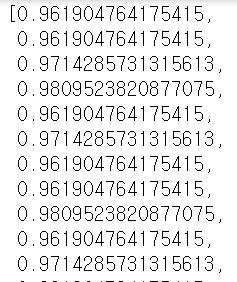
loss, acc = model.evaluate(X_test, y_test)
evaluate에 X_test와 정답인 y_test를 넣어주면 loss와 accuracy를 출력해준다. 정확도는 이전에 머신러닝 모델로 했을 때에 비해 훨씬 개선되었다.
from numpy.random import random
from numpy import round

X_new = round(random([3,4])*10, 2)
print(X_new)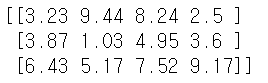
원래는 validation set으로 모델을 검증하고 test set으로 최종 모델을 평가해야 한다. 데이터 셋이 작아서 validation set, test set을 나누지 못하기도 했고, input feature가 4개밖에 되지 않아서 임의로 생성한 숫자들로 test set을 만들어 모델을 평가하겠다. (유의미한 평가는 되지 않겠지만, 임의의 숫자들에 대해 모델이 어떤 답을 내놓는 지만 보겠다!)
y_pred = model.predict(X_new)
print(y_pred)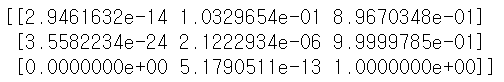
predict는 각 label이 될 확률값을 내놓는 함수이다.
y_pred_classes = model.predict_classes(X_new)
print(y_pred_classes)
predict_classes는 예측한 label을 내놓는 함수이다. 머신러닝 모델에서는 .predict가 라벨값을, .predict_proba가 라벨이 될 확률을 출력했던 것 같은데 여기선 반대로 가는 것 같다.
'딥러닝 > 인공신경망' 카테고리의 다른 글
| LSTM 실습: reuters 예제 (0) | 2021.07.27 |
|---|---|
| LSTM 실습: imdb 예제 (0) | 2021.07.26 |
| CNN 실습: fashion mnist 예제 (0) | 2021.07.23 |
| CNN 실습: mnist 예제 (0) | 2021.07.22 |
| tensorflow, keras 실습: mnist 예제 (2) | 2021.07.22 |


