유튜브 "인과추론의 데이터과학"을 듣고 작성했습니다.
데이터 예시: 푸시메시지가 구매에 미치는 영향

unit fixed effect: time invariant covariates를 모두 통제하여 time invariant covariates를 모두 설명할 수 있음. 즉, time invariants covariate과 perfect collinearity를 가짐
ex) Gender = 1 * D1 + 0 * D2 + 1 * D3 <- time invariant covariate인 Gender은 unit fixed effect인 D1,D2,D3에 의해 perfect collinearity로 설명됨
ex) Age = 20 * D1 + 21 * D2 + 22 * D3
Purchase Amount는 time-varying covariate 이지만 treatment effect를 받기 전/후의 두개의 part로 나뉨. time invariant 부분과 time varying 부분으로 나뉘며, 전자는 unit fixed effect에 의해 흡수된다.
ex) Customer ID = 1에서 Purchase Amount는 day 1,2,3에 50,70,70을 가짐.
day 2에 treatment effect를 받으므로 50,70,70은 각각 50+0, 50+20, 50+20으로 나뉨. 50,50,50은 time invariant 부분으로 unit fixed effect에 의해 흡수되므로 0, 20, 20만 남는다.
Q1. unit fixed effect가 없을 때의 treatment effect
import statsmodels.api as sm
import pandas as pd
import numpy as np

data = pd.DataFrame([
    [1, 1, 0, 50, 1, 20, 'Area A'],
    [1, 2, 1, 70, 1, 20, 'Area A'],
    [1, 3, 1, 70, 1, 20, 'Area A'],
    [2, 1, 0, 10, 0, 21, 'Area A'],
    [2, 2, 1, 30, 0, 21, 'Area A'],
    [2, 3, 1, 50, 0, 21, 'Area A'],
    [3, 1, 0, 30, 1, 22, 'Area B'],
    [3, 2, 0, 20, 1, 22, 'Area B'],
    [3, 3, 0, 10, 1, 22, 'Area B']])
data.columns = ['ID', 'Day', 'PushNotification','PurchaseAmount','Gender','Age', 'Address']

m1 = sm.ols(formula = "PurchaseAmount ~ PushNotification", data = data).fit()
m1.summary()
E(Y1) - E(Y0) = 31
Q2. customer fixed effect 있을 때의 treatment effect
m2 = sm.ols(formula = "PurchaseAmount ~ PushNotification + C(ID)", data = data).fit()
m2.summary()
E(Y1|customer1) - E(Y0|customer1) = (20+20)/2 - 0 = 20
E(Y1|customer2) - E(Y0|customer2) = (20+40)/2 - 0 = 30
-> (20+30)/2 = 25
customer3에서는 Y1이 없기 때문에 treatment effect를 계산할 수 없음
-> customer fixed effect는 within group comparison을 하는 역할을 수행
Q3. customer fixed effect 있을 때, untreated unit을 제외했을때의 treatment effect
m3 = sm.ols(formula = "PurchaseAmount ~ PushNotification + C(ID)", data = data[data.ID.isin([1,2])]).fit()
m3.summary()
customer fixed effect가 있을 때의 treatment effect는 애초에 untreated unit을 제외하기 때문에 Q2와 값이 같음.
regression을 통해 확인해도 같은 결과가 나옴
Q4. customer fixed effect와 day fixed effect가 모두 있을 때의 treatment effect
m4 = sm.ols(formula = "PurchaseAmount ~ PushNotification + C(ID) + C(Day)", data = data).fit()
m4.summary()
customer1의 treatment effect: [(customer1의 treatment 받은 후의 효과 평균) - (customer 3의 treatment 받은 시점 후의 효과 평균)] - [(customer1의 treatment 받기 전의 효과 평균) - (customer 3의 treatment 받은 시점 전의 효과 평균)] = [20-(-15)] - (0-0) = 35
customer2의 treatment effect = 45
-> (35+45)/2 = 40
Q5. customer1은 day3에, customer2는 day2에 treatment effect를 받았다면?
data = pd.DataFrame([
    [1, 1, 0, 50, 1, 20, 'Area A'],
    [1, 2, 0, 70, 1, 20, 'Area A'],
    [1, 3, 1, 70, 1, 20, 'Area A'],
    [2, 1, 0, 10, 0, 21, 'Area A'],
    [2, 2, 1, 30, 0, 21, 'Area A'],
    [2, 3, 1, 50, 0, 21, 'Area A'],
    [3, 1, 0, 30, 1, 22, 'Area B'],
    [3, 2, 0, 20, 1, 22, 'Area B'],
    [3, 3, 0, 10, 1, 22, 'Area B']])
data.columns = ['ID', 'Day', 'PushNotification','PurchaseAmount','Gender','Age', 'Address']

m5 = sm.ols(formula = "PurchaseAmount ~ PushNotification + C(ID) + C(Day)", data = data).fit()
m5.summary()
Staggered Treatment to be addressed later
# Within Matched Applicant Model
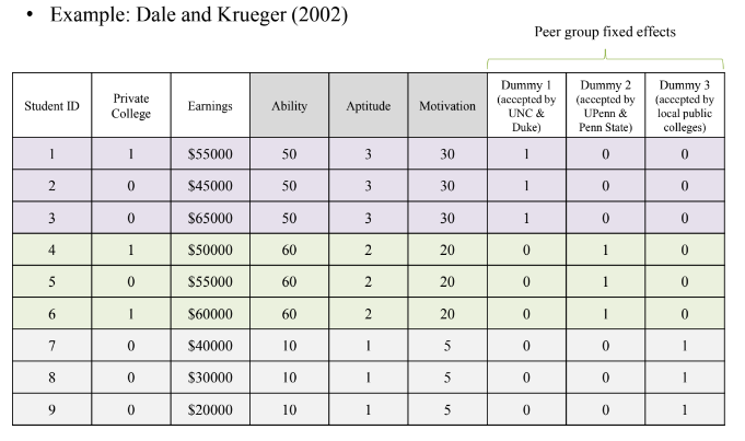
나머지 변수들이 동일한 집단끼리 묶어서 peer group fixed effect을 생성, within group comparison을 수행하여 사립학교 진학이 연봉에 미치는 영향을 분석함
peer group fixed effect가 서로 다른 peer group 간 차이를 흡수함
matching과 비슷한 논리로 작동함
'계량경제학 > 인과추론의 데이터과학' 카테고리의 다른 글
| 인과추론의 다양한 접근법 (0) | 2023.11.21 |
|---|---|
| Matching (0) | 2023.11.19 |
| 인과추론 영역에서의 Data Structure (1) | 2023.11.13 |
| Causal Inference에서의 Regression (2) | 2023.11.09 |
| RCT 실험의 한계점 (0) | 2023.11.09 |


